Your First GWAS Analysis

This tutorial walks you through a complete GWAS analysis from start to finish using Binx.

What You’ll Learn

• How to prepare your data for Binx
• Running a basic GWAS analysis
• Interpreting and visualizing results
• Extracting significant QTLs

Prerequisites

• Binx installed (Installation Guide)
• Genotype data (VCF or dosage format)
• Phenotype data (CSV/TSV)

Sample Data

For this tutorial, we’ll use a tetraploid potato dataset from the R/GWASpoly package.

Download the sample files:

• potato_geno.csv - Genotype data (~9,888 markers, ~1,249 samples)
• potato_pheno.csv - Phenotype data (vine maturity trait)

Citation: Rosyara, U.R., De Jong, W.S., Douches, D.S., & Endelman, J.B. (2016). Software for genome-wide association studies in autopolyploids and its application to potato. The Plant Genome 9(2).

Step 1: Examine Your Data

First, let’s look at our input files:

# Check genotype file structure
head -3 potato_geno.csv

marker,chrom,bp,AF5392-8,AF5393-1,AF5445-2,...
solcap_snp_c2_36608,chr01,508800,1,0,1,...
solcap_snp_c2_36658,chr01,527068,4,3,2,...

# Check phenotype file
head -5 potato_pheno.csv

id,vine.maturity,env
AF5033-13,4.174,Hancock15
AF5153-11,7.674,Hancock15
AF5281-4,4.174,Hancock15
...

Verify sample counts match:

# Count samples in genotype file (columns - 3)
head -1 potato_geno.csv | awk -F',' '{print NF-3, "samples"}'

# Count samples in phenotype file (lines - 1)
wc -l < potato_pheno.csv | awk '{print $1-1, "samples"}'

Step 2: Compute Kinship Matrix (Optional)

The kinship matrix captures genetic relationships. While Binx can auto-generate this using gwaspoly-rs’s set_k() function, computing it separately allows reuse across multiple traits:

binx kinship \
  --geno potato_geno.csv \
  --ploidy 4 \
  --output kinship.tsv

Check the kinship matrix:

# View corner of matrix
head -5 kinship.tsv | cut -f1-5

Diagonal values should be approximately 1.0. Off-diagonal values represent relatedness between samples.

Step 3: Run GWAS

Now run the association analysis:

binx gwas \
  --geno potato_geno.csv \
  --pheno potato_pheno.csv \
  --trait vine.maturity \
  --kinship kinship.tsv \
  --ploidy 4 \
  --models additive \
  --out gwas_results.csv

This will:

1. Load genotypes and phenotypes
2. Match samples between files
3. Fit a mixed model for each marker
4. Output association statistics

Understanding the Output

head gwas_results.csv

marker_id,chrom,pos,model,score,p_value,effect,n_obs,threshold
solcap_snp_c2_36608,chr01,508800,additive,0.64,0.227,0.084,1249,NA
solcap_snp_c2_36658,chr01,527068,additive,0.29,0.508,0.050,1249,NA
...

Key columns:

• score: -log10 transformed p-value (higher = more significant)
• p_value: Probability of seeing this effect by chance
• effect: How much the trait changes per allele dosage unit
• n_obs: Sample size (non-missing)
• threshold: Significance threshold used

Step 4: Calculate Significance Threshold

Determine the significance threshold using M.eff (recommended, accounts for LD):

binx threshold \
  --results gwas_results.csv \
  --method m.eff \
  --geno potato_geno.csv \
  --ploidy 4 \
  --alpha 0.05

Output:

Method: M.eff
Number of tests: 9886
Effective tests (M.eff): 6234
P-value threshold: 8.02e-06
-log10(p) threshold: 5.10

Step 5: Create Visualizations

Manhattan Plot

binx plot \
  --input gwas_results.csv \
  --plot-type manhattan \
  --model additive \
  --threshold 5.1 \
  --title "Vine Maturity GWAS" \
  --output manhattan.png

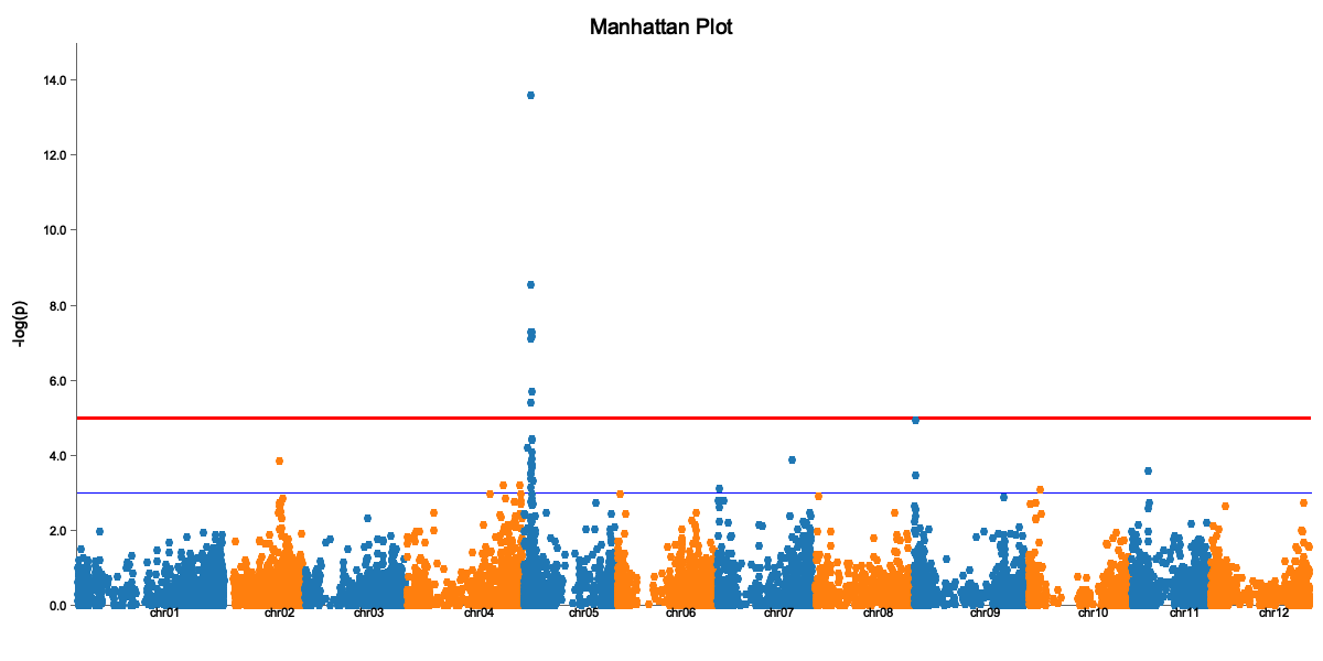
The Manhattan plot shows:

• X-axis: Genomic position (by chromosome)
• Y-axis: -log10(p-value)
• Red line: Significance threshold
• Peaks above the line are significant associations

QQ Plot

binx plot \
  --input gwas_results.csv \
  --plot-type qq \
  --model additive \
  --output qq.png

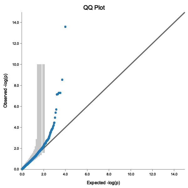
A good QQ plot shows:

• Points following the diagonal line (no inflation)
• Deviation only at the tail (true associations)
• Points within the 95% confidence band

Step 6: Extract Significant QTLs

First, run GWAS with threshold calculation to get a threshold column:

binx gwas \
  --geno potato_geno.csv \
  --pheno potato_pheno.csv \
  --trait vine.maturity \
  --kinship kinship.tsv \
  --ploidy 4 \
  --models additive \
  --threshold m.eff \
  --out gwas_results.csv

Then extract significant QTLs:

binx qtl \
  --input gwas_results.csv \
  --bp-window 5000000 \
  --output significant_qtls.csv

cat significant_qtls.csv

marker_id,chrom,pos,model,score,effect,threshold
solcap_snp_c2_25522,chr05,4561232,additive,6.12,0.52,5.10
PotVar0067031,chr05,5193547,additive,5.89,0.48,5.10

Note: The input file must have a threshold column. Use binx gwas --threshold to generate results with thresholds.

Step 7: Interpret Results

For each significant QTL:

1. Effect size: A positive effect means the alternate allele increases the trait
2. Position: Look up genes near the QTL position
3. MAF: Very rare variants may be false positives

Candidate Gene Analysis

Once you have QTL positions, you can:

• Look up nearby genes in genome browsers
• Check if known candidate genes are in the region
• Examine the LD block around the peak marker

Complete Script

Here’s the full analysis as a script:

#!/bin/bash
set -e

# Configuration (using downloaded sample files)
GENO="potato_geno.csv"
PHENO="potato_pheno.csv"
TRAIT="vine.maturity"
PLOIDY=4
OUTDIR="results"

# Create output directory
mkdir -p $OUTDIR

# Step 1: Compute kinship
echo "Computing kinship matrix..."
binx kinship --geno $GENO --ploidy $PLOIDY --out $OUTDIR/kinship.tsv

# Step 2: Run GWAS with threshold calculation
echo "Running GWAS..."
binx gwas \
  --geno $GENO \
  --pheno $PHENO \
  --trait $TRAIT \
  --kinship $OUTDIR/kinship.tsv \
  --ploidy $PLOIDY \
  --models additive \
  --threshold m.eff \
  --out $OUTDIR/gwas_results.csv

# Step 3: Generate plots
echo "Creating plots..."
binx plot --input $OUTDIR/gwas_results.csv --plot-type manhattan --output $OUTDIR/manhattan.png
binx plot --input $OUTDIR/gwas_results.csv --plot-type qq --output $OUTDIR/qq.png

# Step 4: Extract QTLs
echo "Extracting QTLs..."
binx qtl --input $OUTDIR/gwas_results.csv --bp-window 5000000 --output $OUTDIR/qtls.csv

echo "Done! Results in $OUTDIR/"

Next Steps

• Try different genetic models
• Use LOCO for better p-value calibration
• Analyze multiple environments
• Explore polyploid-specific models

Troubleshooting

“Sample ID mismatch” error

Ensure sample IDs in phenotype file exactly match genotype column headers (case-sensitive).

Inflated QQ plot (points above diagonal)

If your QQ plot shows systematic deviation above the diagonal line:

• Try including principal components (--n-pc 5)
• Check for population structure in your data
• Use LOCO kinship (--loco)

No significant results

• Check if trait is heritable
• Ensure sufficient sample size (>100 recommended)
• Try different genetic models