![]()
Welcome to Binx!
![]()
![]()
Binx is a Rust command-line genomics workbench for diploid and polyploid species. It targets GWAS and related analyses with a familiar UX: fast defaults, explicit inputs, and clear outputs.
What can Binx do?
Binx provides a suite of tools for genomic analysis:
| Command | Description |
|---|---|
binx gwas | GWASpoly-style GWAS with multiple genetic models |
binx kinship | Compute kinship matrix (VanRaden method) |
binx dosage | Estimate genotype dosages from read counts |
binx convert | Convert VCF to other formats |
binx plot | Generate Manhattan, QQ, or LD decay plots |
binx qtl | Identify significant QTLs from GWAS results |
binx threshold | Calculate significance thresholds |
Key Features
- GWASpoly-style GWAS with eight genetic models for polyploids, validated against R/GWASpoly
- Accurate mixed model fitting via rrblup-rs, a Rust implementation of R/rrBLUP’s
mixed.solve - Genotype dosage estimation from VCF or read count data using R/Updog-based algorithms
- Polyploid-aware: supports ploidy levels 2, 4, 6, etc.
- LOCO support: Leave-One-Chromosome-Out analysis
- Multi-environment trials: handles repeated phenotype IDs
Quick Example
# Convert VCF to GWASpoly format
binx convert --vcf samples.vcf.gz --format gwaspoly --output genotypes.tsv

# Run GWAS with multiple genetic models
binx gwas \
  --geno genotypes.tsv \
  --pheno phenotypes.csv \
  --trait yield \
  --ploidy 4 \
  --models additive,general \
  --out gwas_results.csv

# Create a Manhattan plot
binx plot \
  --input gwas_results.csv \
  --plot-type manhattan \
  --model additive \
  --output gwas_manhattan.svg
Getting Started
New to Binx? Start here:
- Installation - Download and install Binx
- Quick Start - Run your first analysis in minutes
- Input Formats - Understand the data formats
Tutorials
Learn Binx through practical examples:
- Your First GWAS Analysis - Step-by-step GWAS walkthrough
- Working with Polyploids - Tetraploid and hexaploid analysis
- Multi-Environment Trials - Handling complex experimental designs
- From VCF to Results - Complete pipeline example
Why Binx?
Binx was created to bring the power of R/GWASpoly and R/rrBLUP to the command line with:
- Speed: Written in Rust for fast execution
- Reproducibility: Explicit parameters and deterministic outputs
- Validation: Results match R implementations to 4-6 decimal places
- Simplicity: No R environment or dependencies required
Getting Help
License
Binx is released under the GPL-3.0 license.
Installation
Binx can be installed via pre-built binaries (recommended) or built from source.
Pre-built Binaries (Recommended)
Download the latest release for your platform from GitHub Releases:
| Platform | Download |
|---|---|
| Linux (x86_64) | binx-linux-x86_64.tar.gz |
| macOS (Intel) | binx-macos-x86_64.tar.gz |
| macOS (Apple Silicon) | binx-macos-aarch64.tar.gz |
Linux Installation
# Download the latest release
curl -LO https://github.com/alex-sandercock/Binx/releases/latest/download/binx-linux-x86_64.tar.gz

# Extract the archive
tar -xzf binx-linux-x86_64.tar.gz

# Verify the installation
./binx --help

# (Optional) Move to a directory in your PATH
mkdir -p ~/bin
mv binx ~/bin/

# Add to PATH if not already present (add to ~/.bashrc or ~/.zshrc)
export PATH="$HOME/bin:$PATH"
macOS Installation
# For Apple Silicon (M1/M2/M3)
curl -LO https://github.com/alex-sandercock/Binx/releases/latest/download/binx-macos-aarch64.tar.gz
tar -xzf binx-macos-aarch64.tar.gz

# For Intel Macs
curl -LO https://github.com/alex-sandercock/Binx/releases/latest/download/binx-macos-x86_64.tar.gz
tar -xzf binx-macos-x86_64.tar.gz

# Verify the installation
./binx --help
Note for macOS users: You may need to allow the binary to run in System Preferences > Security & Privacy if you see a security warning.
Building from Source
Building from source requires the Rust toolchain (cargo + rustc).
Install Rust
If you don’t have Rust installed, get it from rustup.rs:
curl --proto '=https' --tlsv1.2 -sSf https://sh.rustup.rs | sh
source $HOME/.cargo/env
Clone and Build
# Clone the repository
git clone https://github.com/alex-sandercock/Binx.git
cd Binx

# Build in release mode (optimized)
cargo build --release

# The binary will be at target/release/binx
./target/release/binx --help
Install to Cargo Bin Directory
# Install globally via cargo
cargo install --path binx-cli

# Now binx is available anywhere
binx --help
Verifying Your Installation
After installation, verify that Binx is working correctly:
# Check version
binx --version

# View available commands
binx --help

# Check a specific command
binx gwas --help
You should see output similar to:
binx 0.1.0
Rust command-line genomics workbench for diploid and polyploid species

USAGE:
    binx <COMMAND>

COMMANDS:
    gwas       GWASpoly-style GWAS with multiple genetic models
    kinship    Compute kinship matrix (VanRaden method)
    dosage     Estimate genotype dosages from read counts
    convert    Convert VCF to other formats
    plot       Generate Manhattan, QQ, or LD decay plots
    qtl        Identify significant QTLs from GWAS results
    threshold  Calculate significance thresholds
    help       Print this message or the help of the given subcommand(s)
System Requirements
- OS: Linux (x86_64), macOS (Intel or Apple Silicon)
- RAM: Depends on dataset size; typically 4-16 GB for standard GWAS
- Disk: Minimal for the binary; data storage depends on your datasets
Troubleshooting
“Permission denied” error
Make the binary executable:
chmod +x binx
“Command not found” after installation
Ensure the binary location is in your PATH:
# Check where binx is located
which binx

# If not found, add the directory to your PATH
export PATH="$HOME/bin:$PATH"  # or wherever you placed the binary
macOS security warning
If macOS blocks the binary:
- Go to System Preferences > Security & Privacy
- Click “Allow Anyway” next to the Binx message
- Run
binx --helpagain and click “Open” in the dialog
Next Steps
Once installed, proceed to the Quick Start guide to run your first analysis.
Quick Start
This guide will walk you through your first Binx analysis in under 5 minutes.
Overview
A typical Binx workflow looks like this:
VCF file → binx convert → Genotype file ─┐
                                         ├─→ binx gwas → Results → binx plot
                     Phenotype file ─────┘
Step 1: Prepare Your Data
Binx requires two main input files:
Genotype File
A tab-separated file with marker information and sample dosages:
marker_id   chrom   pos     Sample1 Sample2 Sample3
SNP001      1       1000    0       2       4
SNP002      1       2000    1       1       3
SNP003      2       1500    2       2       2
- First three columns:
marker_id,chrom,pos - Remaining columns: sample dosage values (0 to ploidy)
Phenotype File
A CSV/TSV file with sample IDs and trait values:
sample_id,yield,height,env
Sample1,45.2,120,field_A
Sample2,52.1,115,field_A
Sample3,48.7,125,field_B
- First column:
sample_id(must match genotype column headers) - Remaining columns: traits and covariates
Step 2: Convert VCF (if needed)
If your genotypes are in VCF format, convert them first:
binx convert \
  --vcf your_data.vcf.gz \
  --format gwaspoly \
  --output genotypes.tsv
Step 3: Run GWAS
Run a genome-wide association study:
binx gwas \
  --geno genotypes.tsv \
  --pheno phenotypes.csv \
  --trait yield \
  --ploidy 4 \
  --models additive \
  --out gwas_results.csv
Understanding the Parameters
| Parameter | Description |
|---|---|
--geno | Path to genotype file |
--pheno | Path to phenotype file |
--trait | Column name of the trait to analyze |
--ploidy | Ploidy level (2, 4, 6, etc.) |
--models | Genetic models to test |
--out | Output file path |
Step 4: Examine Results
The output CSV contains association results for each marker:
marker_id,chrom,pos,model,score,p_value,effect,n_obs,threshold
SNP001,1,1000,additive,4.49,3.2e-05,0.52,198,5.0
SNP002,1,2000,additive,0.33,0.47,0.08,200,5.0
...
Key columns:
score: -log10 transformed p-value (useful for plotting)p_value: Association p-valueeffect: Effect size estimaten_obs: Sample size (non-missing)threshold: Significance threshold used
Step 5: Visualize Results
Create a Manhattan plot:
binx plot \
  --input gwas_results.csv \
  --plot-type manhattan \
  --model additive \
  --threshold 5 \
  --output manhattan.svg
Create a QQ plot:
binx plot \
  --input gwas_results.csv \
  --plot-type qq \
  --model additive \
  --output qq.svg
Step 6: Identify QTLs
Extract significant QTLs:
binx qtl \
  --input gwas_results.csv \
  --bp-window 10000000 \
  --output significant_qtls.csv
Complete Example Script
Here’s a complete analysis pipeline you can adapt:
#!/bin/bash

# Define input files
VCF="data/samples.vcf.gz"
PHENO="data/phenotypes.csv"
TRAIT="yield"
PLOIDY=4

# Create output directory
mkdir -p results

# Step 1: Convert VCF to Binx format
binx convert \
  --vcf $VCF \
  --format gwaspoly \
  --output results/genotypes.tsv

# Step 2: Run GWAS with multiple models
binx gwas \
  --geno results/genotypes.tsv \
  --pheno $PHENO \
  --trait $TRAIT \
  --ploidy $PLOIDY \
  --models additive,general,1-dom,2-dom \
  --out results/gwas_results.csv

# Step 3: Generate plots
binx plot \
  --input results/gwas_results.csv \
  --plot-type manhattan \
  --model additive \
  --threshold 5 \
  --output results/manhattan.svg

binx plot \
  --input results/gwas_results.csv \
  --plot-type qq \
  --model additive \
  --output results/qq.svg

# Step 4: Extract QTLs
binx qtl \
  --input results/gwas_results.csv \
  --bp-window 10000000 \
  --output results/qtls.csv

echo "Analysis complete! Results in results/"
Next Steps
- Learn about Input Formats in detail
- Explore Genetic Models available in Binx
- Follow the First GWAS Tutorial for a more detailed walkthrough
- Check the Command Reference for all options
Input Formats
This page describes the input file formats that Binx accepts.
Genotype File
The genotype file contains marker information and dosage values for each sample.
Format Specification
- File type: TSV (tab-separated) or CSV (comma-separated)
- Header: Required (first row)
- Columns:
- Column 1:
marker_id- unique marker identifier - Column 2:
chrom- chromosome name/number - Column 3:
pos- base pair position (integer) - Columns 4+: Sample dosage values
- Column 1:
Example
marker_id	chrom	pos	Sample1	Sample2	Sample3	Sample4
SNP_1_1000	1	1000	0	2	4	1
SNP_1_2000	1	2000	1	1	3	2
SNP_1_3500	1	3500	4	0	2	2
SNP_2_500	2	500	2	2	2	3
SNP_2_1200	2	1200	0	1	1	0
Dosage Values
Dosage values represent the count of the alternate allele:
| Ploidy | Valid Values | Meaning |
|---|---|---|
| Diploid (2) | 0, 1, 2 | 0=AA, 1=AB, 2=BB |
| Tetraploid (4) | 0, 1, 2, 3, 4 | 0=AAAA … 4=BBBB |
| Hexaploid (6) | 0, 1, 2, 3, 4, 5, 6 | 0=AAAAAA … 6=BBBBBB |
Missing Values
Missing genotypes can be encoded as:
NA- Empty cell
.
marker_id	chrom	pos	Sample1	Sample2	Sample3
SNP001	1	1000	0	NA	4
SNP002	1	2000	1	.	3
SNP003	1	3500		2	2
Converting from VCF
Use binx convert to create a genotype file from VCF:
binx convert \
  --vcf input.vcf.gz \
  --format gwaspoly \
  --output genotypes.tsv
Phenotype File
The phenotype file contains trait values and optional covariates for each sample.
Format Specification
- File type: TSV or CSV
- Header: Required (first row)
- Columns:
- Column 1:
sample_id- must match genotype file column headers - Remaining columns: traits and/or covariates
- Column 1:
Example
sample_id,yield,height,flowering_date,environment,block
Sample1,45.2,120,156,field_A,1
Sample2,52.1,115,148,field_A,2
Sample3,48.7,125,152,field_B,1
Sample4,51.3,118,150,field_B,2
Trait Values
- Numeric values for quantitative traits
- Can include
NAor empty cells for missing values
Covariates
Binx automatically detects covariate types:
| Type | Detection | Example |
|---|---|---|
| Numeric | All values are numbers | height, age |
| Factor | Contains non-numeric values | environment, block |
Factor covariates are automatically dummy-coded during analysis.
Multi-Environment Trials
For repeated measurements (same sample in multiple environments), repeat the sample ID:
sample_id,yield,environment,replicate
Sample1,45.2,field_A,1
Sample1,47.8,field_A,2
Sample1,44.1,field_B,1
Sample2,52.1,field_A,1
Sample2,50.3,field_A,2
Kinship Matrix
The kinship matrix represents genetic relationships between samples.
Format Specification
- File type: TSV or CSV
- Structure: Square symmetric matrix
- Header: Sample IDs
- Row names: Sample IDs (first column)
Example
sample_id	Sample1	Sample2	Sample3	Sample4
Sample1	1.000	0.250	0.125	0.150
Sample2	0.250	1.000	0.200	0.180
Sample3	0.125	0.200	1.000	0.220
Sample4	0.150	0.180	0.220	1.000
Computing a Kinship Matrix
Use binx kinship to compute from genotypes:
binx kinship \
  --geno genotypes.tsv \
  --ploidy 4 \
  --method vanraden \
  --out kinship.tsv
Kinship Methods
| Method | Description |
|---|---|
vanraden | VanRaden (2008) method 1 (default) |
gwaspoly | GWASpoly-style kinship |
VCF Files
Binx can import VCF (Variant Call Format) files via binx convert.
Supported Features
- Gzipped (
.vcf.gz) and uncompressed (.vcf) files - Diploid and polyploid genotypes
- GT (genotype) and AD (allelic depth) fields
Example Conversion
# Convert VCF to GWASpoly format (using GT field)
binx convert \
  --vcf input.vcf.gz \
  --format gwaspoly \
  --output genotypes.tsv

# Convert VCF to allele depths for dosage estimation (using AD field)
binx convert \
  --vcf input.vcf.gz \
  --format csv \
  --output allele_depths.csv
File Tips
Sample ID Matching
Sample IDs in the phenotype file must exactly match the column headers in the genotype file:
# Genotype file header:
marker_id  chrom  pos  Sample_001  Sample_002  Sample_003

# Phenotype file:
sample_id,yield
Sample_001,45.2    ✓ matches
Sample_002,52.1    ✓ matches
sample_003,48.7    ✗ case mismatch!
Chromosome Naming
Chromosome names can be:
- Numeric:
1,2,3, … - String:
chr1,Chr1,chromosome1
Be consistent within your genotype file.
Large Files
For very large datasets:
- Use compressed VCF: Keep VCF files gzipped
- Filter early: Apply MAF and missing data filters during conversion
- Subset chromosomes: Analyze one chromosome at a time if needed
Validation
Check your files before analysis:
# Check genotype file structure
head -5 genotypes.tsv

# Count samples and markers
awk 'NR==1 {print "Samples:", NF-3} END {print "Markers:", NR-1}' genotypes.tsv

# Check phenotype file
head phenotypes.csv
wc -l phenotypes.csv
Your First GWAS Analysis
This tutorial walks you through a complete GWAS analysis from start to finish using Binx.
What You’ll Learn
- How to prepare your data for Binx
- Running a basic GWAS analysis
- Interpreting and visualizing results
- Extracting significant QTLs
Prerequisites
- Binx installed (Installation Guide)
- Genotype data (VCF or dosage format)
- Phenotype data (CSV/TSV)
Sample Data
For this tutorial, we’ll use a tetraploid potato dataset from the R/GWASpoly package.
Download the sample files:
- potato_geno.csv - Genotype data (~9,888 markers, ~1,249 samples)
- potato_pheno.csv - Phenotype data (vine maturity trait)
Citation: Rosyara, U.R., De Jong, W.S., Douches, D.S., & Endelman, J.B. (2016). Software for genome-wide association studies in autopolyploids and its application to potato. The Plant Genome 9(2).
Step 1: Examine Your Data
First, let’s look at our input files:
# Check genotype file structure
head -3 potato_geno.csv
marker,chrom,bp,AF5392-8,AF5393-1,AF5445-2,...
solcap_snp_c2_36608,chr01,508800,1,0,1,...
solcap_snp_c2_36658,chr01,527068,4,3,2,...
# Check phenotype file
head -5 potato_pheno.csv
id,vine.maturity,env
AF5033-13,4.174,Hancock15
AF5153-11,7.674,Hancock15
AF5281-4,4.174,Hancock15
...
Verify sample counts match:
# Count samples in genotype file (columns - 3)
head -1 potato_geno.csv | awk -F',' '{print NF-3, "samples"}'

# Count samples in phenotype file (lines - 1)
wc -l < potato_pheno.csv | awk '{print $1-1, "samples"}'
Step 2: Compute Kinship Matrix (Optional)
The kinship matrix captures genetic relationships. While Binx can auto-generate this using gwaspoly-rs’s set_k() function, computing it separately allows reuse across multiple traits:
binx kinship \
  --geno potato_geno.csv \
  --ploidy 4 \
  --output kinship.tsv
Check the kinship matrix:
# View corner of matrix
head -5 kinship.tsv | cut -f1-5
Diagonal values should be approximately 1.0. Off-diagonal values represent relatedness between samples.
Step 3: Run GWAS
Now run the association analysis:
binx gwas \
  --geno potato_geno.csv \
  --pheno potato_pheno.csv \
  --trait vine.maturity \
  --kinship kinship.tsv \
  --ploidy 4 \
  --models additive \
  --out gwas_results.csv
This will:
- Load genotypes and phenotypes
- Match samples between files
- Fit a mixed model for each marker
- Output association statistics
Understanding the Output
head gwas_results.csv
marker_id,chrom,pos,model,score,p_value,effect,n_obs,threshold
solcap_snp_c2_36608,chr01,508800,additive,0.64,0.227,0.084,1249,NA
solcap_snp_c2_36658,chr01,527068,additive,0.29,0.508,0.050,1249,NA
...
Key columns:
score: -log10 transformed p-value (higher = more significant)p_value: Probability of seeing this effect by chanceeffect: How much the trait changes per allele dosage unitn_obs: Sample size (non-missing)threshold: Significance threshold used
Step 4: Calculate Significance Threshold
Determine the significance threshold using M.eff (recommended, accounts for LD):
binx threshold \
  --results gwas_results.csv \
  --method m.eff \
  --geno potato_geno.csv \
  --ploidy 4 \
  --alpha 0.05
Output:
Method: M.eff
Number of tests: 9886
Effective tests (M.eff): 6234
P-value threshold: 8.02e-06
-log10(p) threshold: 5.10
Step 5: Create Visualizations
Manhattan Plot
binx plot \
  --input gwas_results.csv \
  --plot-type manhattan \
  --model additive \
  --threshold 5.1 \
  --title "Vine Maturity GWAS" \
  --output manhattan.png
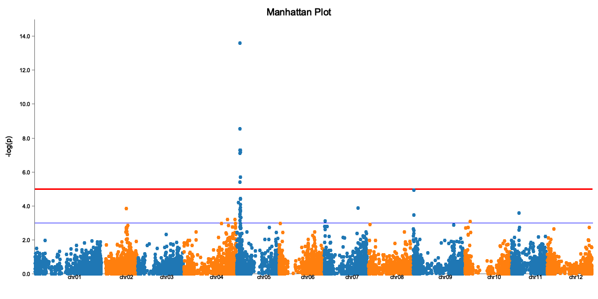
The Manhattan plot shows:
- X-axis: Genomic position (by chromosome)
- Y-axis: -log10(p-value)
- Red line: Significance threshold
- Peaks above the line are significant associations
QQ Plot
binx plot \
  --input gwas_results.csv \
  --plot-type qq \
  --model additive \
  --output qq.png
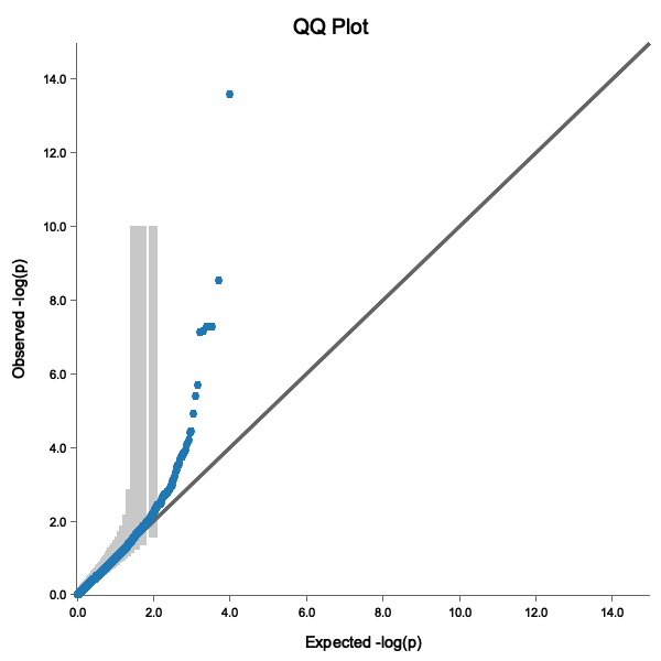
A good QQ plot shows:
- Points following the diagonal line (no inflation)
- Deviation only at the tail (true associations)
- Points within the 95% confidence band
Step 6: Extract Significant QTLs
First, run GWAS with threshold calculation to get a threshold column:
binx gwas \
  --geno potato_geno.csv \
  --pheno potato_pheno.csv \
  --trait vine.maturity \
  --kinship kinship.tsv \
  --ploidy 4 \
  --models additive \
  --threshold m.eff \
  --out gwas_results.csv
Then extract significant QTLs:
binx qtl \
  --input gwas_results.csv \
  --bp-window 5000000 \
  --output significant_qtls.csv
cat significant_qtls.csv
marker_id,chrom,pos,model,score,effect,threshold
solcap_snp_c2_25522,chr05,4561232,additive,6.12,0.52,5.10
PotVar0067031,chr05,5193547,additive,5.89,0.48,5.10
Note: The input file must have a
thresholdcolumn. Usebinx gwas --thresholdto generate results with thresholds.
Step 7: Interpret Results
For each significant QTL:
- Effect size: A positive effect means the alternate allele increases the trait
- Position: Look up genes near the QTL position
- MAF: Very rare variants may be false positives
Candidate Gene Analysis
Once you have QTL positions, you can:
- Look up nearby genes in genome browsers
- Check if known candidate genes are in the region
- Examine the LD block around the peak marker
Complete Script
Here’s the full analysis as a script:
#!/bin/bash
set -e

# Configuration (using downloaded sample files)
GENO="potato_geno.csv"
PHENO="potato_pheno.csv"
TRAIT="vine.maturity"
PLOIDY=4
OUTDIR="results"

# Create output directory
mkdir -p $OUTDIR

# Step 1: Compute kinship
echo "Computing kinship matrix..."
binx kinship --geno $GENO --ploidy $PLOIDY --out $OUTDIR/kinship.tsv

# Step 2: Run GWAS with threshold calculation
echo "Running GWAS..."
binx gwas \
  --geno $GENO \
  --pheno $PHENO \
  --trait $TRAIT \
  --kinship $OUTDIR/kinship.tsv \
  --ploidy $PLOIDY \
  --models additive \
  --threshold m.eff \
  --out $OUTDIR/gwas_results.csv

# Step 3: Generate plots
echo "Creating plots..."
binx plot --input $OUTDIR/gwas_results.csv --plot-type manhattan --output $OUTDIR/manhattan.png
binx plot --input $OUTDIR/gwas_results.csv --plot-type qq --output $OUTDIR/qq.png

# Step 4: Extract QTLs
echo "Extracting QTLs..."
binx qtl --input $OUTDIR/gwas_results.csv --bp-window 5000000 --output $OUTDIR/qtls.csv

echo "Done! Results in $OUTDIR/"
Next Steps
- Try different genetic models
- Use LOCO for better p-value calibration
- Analyze multiple environments
- Explore polyploid-specific models
Troubleshooting
“Sample ID mismatch” error
Ensure sample IDs in phenotype file exactly match genotype column headers (case-sensitive).
Inflated QQ plot (points above diagonal)
If your QQ plot shows systematic deviation above the diagonal line:
- Try including principal components (
--n-pc 5) - Check for population structure in your data
- Use LOCO kinship (
--loco)
No significant results
- Check if trait is heritable
- Ensure sufficient sample size (>100 recommended)
- Try different genetic models
Working with Polyploids
This tutorial covers GWAS analysis in polyploid species using Binx’s specialized genetic models.
Introduction to Polyploid GWAS
Polyploid species (tetraploids, hexaploids, etc.) have more than two copies of each chromosome, which creates unique challenges and opportunities for GWAS:
- More allele combinations: A tetraploid has 5 possible genotypes per locus (0-4 copies)
- Complex inheritance: Dominance relationships are more nuanced
- Higher genetic diversity: More combinations can influence traits
Binx implements the GWASpoly framework, which models various forms of allele dosage effects.
Genetic Models for Polyploids
Understanding Dosage Effects
In a tetraploid, the five genotypes (AAAA, AAAB, AABB, ABBB, BBBB) can affect traits differently:
| Model | Assumption | Best For |
|---|---|---|
| Additive | Linear dosage effect | Quantitative traits with dosage dependence |
| General | No assumption (4 df) | Unknown inheritance; hypothesis generation |
| Simplex dominant | One B allele is sufficient | Traits with low-dosage dominance |
| Duplex dominant | Two B alleles are sufficient | Intermediate dominance |
Choosing Models
Start with additive + general:
binx gwas \
  --geno genotypes.tsv \
  --pheno phenotypes.csv \
  --trait yield \
  --ploidy 4 \
  --models additive,general \
  --out results.csv
- Additive captures dosage-dependent effects
- General captures any pattern (exploratory)
Then investigate specific dominance patterns:
binx gwas \
  --geno genotypes.tsv \
  --pheno phenotypes.csv \
  --trait disease_resistance \
  --ploidy 4 \
  --models additive,1-dom,2-dom \
  --out results.csv
Example: Tetraploid Potato GWAS
Let’s analyze a tetraploid potato dataset for tuber yield.
Step 1: Verify Ploidy in Data
Check that dosage values are appropriate:
# Find max dosage value
awk -F'\t' 'NR>1 {for(i=4;i<=NF;i++) if($i>max) max=$i} END {print "Max dosage:", max}' genotypes.tsv
For tetraploid data, max should be 4.
Step 2: Compute Polyploid Kinship
binx kinship \
  --geno genotypes.tsv \
  --ploidy 4 \
  --output kinship.tsv
Step 3: Run Multi-Model GWAS
binx gwas \
  --geno genotypes.tsv \
  --pheno phenotypes.csv \
  --trait yield \
  --kinship kinship.tsv \
  --ploidy 4 \
  --models additive,general,1-dom,2-dom \
  --loco \
  --out gwas_results.csv
Step 4: Compare Models
Extract results by model:
# Count significant hits per model (threshold -log10p > 5)
awk -F',' 'NR>1 && $8>5 {count[$4]++} END {for(m in count) print m, count[m]}' gwas_results.csv
Create model-specific Manhattan plots:
for model in additive general 1-dom-ref 1-dom-alt 2-dom-ref 2-dom-alt; do
  binx plot \
    --input gwas_results.csv \
    --plot-type manhattan \
    --model $model \
    --threshold 5 \
    --title "Yield GWAS - $model model" \
    --output manhattan_${model}.svg
done
Step 5: Interpret Model-Specific Results
If a QTL is significant under:
- Additive only: Dosage-dependent effect (each additional allele adds to trait)
- 1-dom only: Presence/absence effect (one copy is enough)
- General but not additive: Complex dominance pattern
- Multiple models: Robust association, exact inheritance unclear
Hexaploid Analysis
For hexaploid species (ploidy=6), the same workflow applies:
binx gwas \
  --geno genotypes.tsv \
  --pheno phenotypes.csv \
  --trait yield \
  --ploidy 6 \
  --models additive,general \
  --out results.csv
Hexaploids have 7 possible dosage values (0-6) and even more complex dominance patterns.
Tips for Polyploid GWAS
Sample Size
Polyploids need larger sample sizes due to:
- More parameters in genetic models
- Lower power to detect effects
- Recommendation: 200+ samples for tetraploids
MAF Filtering
Be careful with MAF filtering in polyploids:
# More lenient MAF for polyploids
binx gwas \
  --geno genotypes.tsv \
  --pheno phenotypes.csv \
  --trait yield \
  --ploidy 4 \
  --min-maf 0.02 \
  --out results.csv
Low-frequency variants in polyploids can still be informative.
Interpreting Effect Sizes
Effect sizes are reported for single-parameter models:
- Additive: Effect per dosage unit (in trait units)
- Dominance models (1-dom, 2-dom, etc.): Effect of the dominant group vs reference
Note: The general model does not report effect sizes because it performs a joint test of multiple parameters. Use it for detecting associations with complex inheritance, then follow up with specific models to estimate effects.
Diploidized Analysis
Sometimes you want to treat polyploid data as diploid-like:
binx gwas \
  --geno genotypes.tsv \
  --pheno phenotypes.csv \
  --trait yield \
  --ploidy 4 \
  --models diplo-additive,diplo-general \
  --out results.csv
This collapses dosage categories:
- 0 → “AA-like”
- 1, 2, 3 → “AB-like” (heterozygotes)
- 4 → “BB-like”
Useful when expecting diploid-like inheritance in a polyploid.
See Also
- Genetic Models Reference - Detailed model descriptions
- Multi-Environment Trials - Complex experimental designs
- Validation - Accuracy compared to R/GWASpoly
Multi-Environment Trials
This tutorial covers GWAS analysis with repeated measurements across multiple environments.
Overview
Multi-environment trials (MET) are common in plant breeding where the same genotypes are evaluated across multiple locations, years, or treatments. Binx handles these designs through:
- Repeated sample IDs in phenotype files
- Environment as a covariate
- Appropriate mixed model handling
Data Structure
Your phenotype file can include repeated measurements:
sample_id,yield,environment,replicate
Sample001,45.2,field_A,1
Sample001,47.8,field_A,2
Sample001,44.1,field_B,1
Sample002,52.1,field_A,1
Sample002,50.3,field_A,2
Running MET GWAS
binx gwas \
  --geno genotypes.tsv \
  --pheno phenotypes.csv \
  --trait yield \
  --covariates environment \
  --ploidy 4 \
  --out results.csv
Analyzing G×E Interactions
Coming soon: Detailed tutorial on G×E analysis
See Also
From VCF to Results
A complete pipeline tutorial showing a full workflow from raw VCF data to GWAS results.
Overview
This tutorial demonstrates the full Binx workflow:
- Convert VCF to Binx format
- Quality control and filtering
- Compute kinship matrix
- Run GWAS with multiple models
- Generate visualizations
- Extract and interpret QTLs
Complete Pipeline Script
#!/bin/bash
set -e

# === Configuration ===
VCF="raw_data/variants.vcf.gz"
PHENO="raw_data/phenotypes.csv"
TRAIT="yield"
PLOIDY=4
OUTDIR="results"

mkdir -p $OUTDIR

# === Step 1: Convert VCF ===
echo "Converting VCF..."
binx convert \
  --vcf $VCF \
  --format gwaspoly \
  --output $OUTDIR/genotypes.tsv

# === Step 2: Compute Kinship ===
echo "Computing kinship..."
binx kinship \
  --geno $OUTDIR/genotypes.tsv \
  --ploidy $PLOIDY \
  --output $OUTDIR/kinship.tsv

# === Step 3: Run GWAS ===
echo "Running GWAS..."
binx gwas \
  --geno $OUTDIR/genotypes.tsv \
  --pheno $PHENO \
  --trait $TRAIT \
  --kinship $OUTDIR/kinship.tsv \
  --ploidy $PLOIDY \
  --models additive,general \
  --loco \
  --threshold bonferroni \
  --out $OUTDIR/gwas_results.csv

# === Step 4: Visualize ===
echo "Creating plots..."
binx plot \
  --input $OUTDIR/gwas_results.csv \
  --plot-type manhattan \
  --model additive \
  --output $OUTDIR/manhattan.svg

binx plot \
  --input $OUTDIR/gwas_results.csv \
  --plot-type qq \
  --model additive \
  --output $OUTDIR/qq.svg

# === Step 5: Extract QTLs ===
echo "Extracting QTLs..."
binx qtl \
  --input $OUTDIR/gwas_results.csv \
  --bp-window 5000000 \
  --output $OUTDIR/qtls.csv

echo "Done! Results in $OUTDIR/"
See Also
Command Overview
Binx provides a suite of commands for genomic analysis. Each command is designed to handle a specific task in the analysis pipeline.
Command Structure
All Binx commands follow the pattern:
binx <command> [options]
Get help for any command with --help:
binx --help           # List all commands
binx gwas --help      # Help for specific command
Available Commands
Analysis Commands
| Command | Description | Primary Use |
|---|---|---|
gwas | Genome-wide association study | Identify trait-associated markers |
kinship | Compute kinship matrix | Account for population structure |
dosage | Estimate genotype dosages | Process read count data |
Utility Commands
| Command | Description | Primary Use |
|---|---|---|
convert | Convert file formats | Prepare VCF data for analysis |
plot | Generate visualizations | Create Manhattan/QQ plots |
qtl | Extract QTLs | Identify significant loci |
threshold | Calculate thresholds | Determine significance cutoffs |
Typical Workflows
Basic GWAS Pipeline
# 1. Convert VCF to Binx format
binx convert --vcf data.vcf.gz --output geno.tsv --format gwaspoly

# 2. Compute kinship matrix
binx kinship --geno geno.tsv --ploidy 4 --out kinship.tsv

# 3. Run GWAS
binx gwas --geno geno.tsv --pheno pheno.csv --trait yield \
          --kinship kinship.tsv --ploidy 4 --out results.csv

# 4. Visualize results
binx plot --input results.csv --output manhattan.svg --plot-type manhattan
With Dosage Estimation from VCF
# 1. Estimate dosages from VCF with allele depths
binx dosage --vcf data.vcf.gz --ploidy 4 --output geno.tsv --format gwaspoly

# 2. Continue with GWAS...
binx gwas --geno geno.tsv --pheno pheno.csv --out results.csv --trait yield --ploidy 4
Common Options
These options are available across multiple commands:
| Option | Description |
|---|---|
--help, -h | Display help information |
--version, -V | Display version information (top-level only) |
--verbose | Enable verbose output (where applicable) |
--threads | Number of threads (where applicable) |
--output or --out | Output file path (varies by command) |
Exit Codes
| Code | Meaning |
|---|---|
0 | Success |
1 | Error (invalid arguments, file not found, processing error, etc.) |
Next Steps
Explore individual command documentation:
- binx gwas - The main GWAS command
- binx kinship - Kinship matrix computation
- binx convert - File format conversion
binx gwas
Perform genome-wide association studies (GWAS) using GWASpoly-style methods with support for multiple genetic models.
Synopsis
binx gwas --geno <FILE> --pheno <FILE> --out <FILE> --trait <NAME> --ploidy <INT> [OPTIONS]
Description
The gwas command performs association analysis between genetic markers and phenotypic traits. It implements the statistical methods from GWASpoly (Rosyara et al., 2016) and rrBLUP (Endelman, 2011), supporting both diploid and polyploid species.
Key features:
- Multiple genetic models for polyploid analysis
- Mixed model framework (K model, P+K model)
- Leave-One-Chromosome-Out (LOCO) kinship
- Support for covariates and multi-environment trials
Required Arguments
| Argument | Description |
|---|---|
--geno <FILE> | Genotype dosage file (TSV: marker, chr, pos, samples…). Missing values (NA) are imputed with marker mean. |
--pheno <FILE> | Phenotype file (CSV: sample_id, traits…) |
--out <FILE> | Output results CSV |
--trait <NAME> | Trait name to analyze |
--ploidy <INT> | Ploidy level (e.g., 2, 4, 6) |
Missing Value Handling: Missing genotype values (NA) are automatically imputed with the marker mean. This matches the default behavior of R/GWASpoly.
Options
Method
| Option | Default | Description |
|---|---|---|
--method <METHOD> | gwaspoly | GWAS method to use |
Analysis Options
| Option | Default | Description |
|---|---|---|
--models <LIST> | additive,general | Genetic models to test (comma-separated) |
--kinship <FILE> | - | Pre-computed kinship matrix TSV (optional; auto-generated if omitted) |
--loco | false | Use Leave-One-Chromosome-Out kinship |
--n-pc <INT> | 0 | Number of principal components to include as fixed effects (P+K model) |
--covariates <LIST> | - | Covariates from phenotype file (comma-separated) |
Note: If
--kinshipis not provided, Binx automatically computes a kinship matrix using gwaspoly-rs’sset_k()function (equivalent to R/GWASpoly’sset.K()). Pre-computing withbinx kinshipis recommended when running multiple traits to avoid redundant computation.
QC Filters
| Option | Default | Description |
|---|---|---|
--min-maf <FLOAT> | 0.0 | Minimum minor allele frequency (0.0-0.5) |
--max-geno-freq <FLOAT> | 0.0 | Maximum genotype frequency (0.0-1.0, 0=auto) |
--allow-missing-samples | false | Allow samples in geno but not in pheno |
Threshold Options
| Option | Default | Description |
|---|---|---|
--threshold <METHOD> | - | Threshold method: m.eff (recommended), bonferroni, or fdr |
--alpha <FLOAT> | 0.05 | Significance level |
Output Options
| Option | Default | Description |
|---|---|---|
--plot <TYPE> | - | Generate plots: manhattan, qq, or both |
--plot-output <FILE> | - | Custom path for plot files |
--parallel | false | Use parallel marker testing |
Genetic Models
The --models option accepts the following values. These match R/GWASpoly’s gene action models (Rosyara et al., 2016).
For Diploids (ploidy=2)
| Model | Description | Encoding | df |
|---|---|---|---|
additive | Linear dosage effect | 0, 1, 2 | 1 |
general | Separate effect per dosage | dummy coded | 2 |
1-dom | Dominant (tests both ref and alt) | — | 1 each |
1-dom-ref | Dominant (ref group distinct) | 0, 1, 1 | 1 |
1-dom-alt | Dominant (alt group distinct) | 0, 0, 1 | 1 |
For Tetraploids (ploidy=4)
| Model | Description | Encoding | df |
|---|---|---|---|
additive | Linear dosage effect | 0, 1, 2, 3, 4 | 1 |
general | Separate effect per dosage | dummy coded | 4 |
1-dom | Simplex dominant (tests both ref and alt) | — | 1 each |
1-dom-ref | Simplex dominant (ref group distinct) | 0, 1, 1, 1, 1 | 1 |
1-dom-alt | Simplex dominant (alt group distinct) | 0, 0, 0, 0, 1 | 1 |
2-dom | Duplex dominant (tests both ref and alt) | — | 1 each |
2-dom-ref | Duplex dominant (ref side distinct) | 0, 0, 1, 1, 1 | 1 |
2-dom-alt | Duplex dominant (alt side distinct) | 0, 0, 0, 1, 1 | 1 |
diplo-general | Diploidized general (hets collapsed) | dummy coded | 2 |
diplo-additive | Diploidized additive (hets = 0.5) | 0, 0.5, 0.5, 0.5, 1 | 1 |
Model Expansion
Like R/GWASpoly, specifying 1-dom automatically tests both 1-dom-ref and 1-dom-alt. Similarly, 2-dom expands to both 2-dom-ref and 2-dom-alt. Use the specific -ref or -alt variants if you only want one direction.
Using Multiple Models
Specify multiple models separated by commas:
binx gwas --models additive,general,1-dom,2-dom ...
See Genetic Models Reference for detailed explanations.
Examples
Basic GWAS
binx gwas \
  --geno genotypes.tsv \
  --pheno phenotypes.csv \
  --trait yield \
  --ploidy 4 \
  --out results.csv
With Pre-computed Kinship
# First compute kinship
binx kinship --geno genotypes.tsv --out kinship.tsv

# Then run GWAS
binx gwas \
  --geno genotypes.tsv \
  --pheno phenotypes.csv \
  --trait yield \
  --kinship kinship.tsv \
  --ploidy 4 \
  --out results.csv
LOCO Analysis
Leave-One-Chromosome-Out reduces proximal contamination:
binx gwas \
  --geno genotypes.tsv \
  --pheno phenotypes.csv \
  --trait yield \
  --ploidy 4 \
  --loco \
  --out results.csv
With Covariates and PCs
binx gwas \
  --geno genotypes.tsv \
  --pheno phenotypes.csv \
  --trait yield \
  --covariates environment,block \
  --n-pc 3 \
  --ploidy 4 \
  --out results.csv
Multiple Genetic Models
binx gwas \
  --geno genotypes.tsv \
  --pheno phenotypes.csv \
  --trait yield \
  --ploidy 4 \
  --models additive,general,1-dom,2-dom \
  --out results.csv
With Threshold Calculation
binx gwas \
  --geno genotypes.tsv \
  --pheno phenotypes.csv \
  --trait yield \
  --ploidy 4 \
  --models additive,general \
  --threshold m.eff \
  --out results.csv
With Plots
binx gwas \
  --geno genotypes.tsv \
  --pheno phenotypes.csv \
  --trait yield \
  --ploidy 4 \
  --kinship kinship.tsv \
  --plot both \
  --out results.csv
Output Format
The output file contains the following columns:
| Column | Description |
|---|---|
marker_id | Marker identifier |
chrom | Chromosome |
pos | Base pair position |
model | Genetic model used |
score | -log10(p-value) |
p_value | Association p-value |
effect | Effect size estimate |
n_obs | Sample size (non-missing) |
threshold | Significance threshold used |
Example Output
marker_id,chrom,pos,model,score,p_value,effect,n_obs,threshold
SNP_1_1000,1,1000,additive,4.49,3.21e-05,0.523,198,5.0
SNP_1_2000,1,2000,additive,0.33,0.469,0.081,200,5.0
SNP_1_3500,1,3500,additive,2.84,1.45e-03,-0.312,195,5.0
Statistical Details
Mixed Model
The GWAS uses a linear mixed model:
y = Xβ + Zu + e
Where:
y= phenotype vectorX= fixed effects design matrix (intercept, covariates, marker)β= fixed effectsZ= random effects design matrixu ~ N(0, Kσ²ᵤ)= random polygenic effectsK= kinship matrixe ~ N(0, Iσ²ₑ)= residual errors
P+K Model
When --n-pc is specified, principal components are included as fixed effects to account for population structure (P+K model).
LOCO
With --loco, the kinship matrix is recalculated for each chromosome, excluding markers on the chromosome being tested. This prevents the tested marker from influencing its own significance through the kinship matrix.
Tips and Best Practices
-
Choose appropriate models: For autopolyploids, start with
additiveandgeneral. The general model captures complex dominance patterns but uses more degrees of freedom. -
Use LOCO for accurate p-values: LOCO prevents proximal contamination and generally provides better-calibrated p-values.
-
Pre-compute kinship for efficiency: If running multiple traits, compute the kinship matrix once and reuse it.
-
Filter markers: Use
--min-mafto remove rare variants that have low power. -
Calculate significance thresholds: Use
--threshold m.effto compute the effective number of tests threshold, which accounts for LD between markers. -
Generate plots directly: Use
--plot bothto generate Manhattan and QQ plots automatically after GWAS completes. -
Use parallel mode: For large datasets,
--parallelcan speed up marker testing.
See Also
- binx kinship - Compute kinship matrices
- binx plot - Visualize GWAS results
- binx qtl - Extract significant QTLs
- Genetic Models Reference
binx kinship
Compute kinship (genomic relationship) matrices from genotype data.
Synopsis
binx kinship --geno <FILE> --ploidy <INT> --out <FILE> [OPTIONS]
Description
The kinship command computes a genomic relationship matrix (GRM) from marker dosage data. The kinship matrix captures genetic similarity between individuals and is used in GWAS to account for population structure and relatedness.
When to use: While
binx gwasauto-generates a kinship matrix if not provided (using gwaspoly-rs’sset_k()), pre-computing withbinx kinshipis recommended when:
- Running GWAS on multiple traits (avoids recomputation)
- You need a specific kinship method (VanRaden vs GWASpoly)
- You want to inspect or reuse the kinship matrix
Required Arguments
| Argument | Description |
|---|---|
--geno <FILE> | Path to genotype file (TSV/CSV with dosages) |
--ploidy <INT> | Ploidy level (e.g., 2, 4, 6) |
--out <FILE> | Output file path |
Options
| Option | Default | Description |
|---|---|---|
--method <METHOD> | vanraden | Kinship method: vanraden or gwaspoly |
Methods
VanRaden (default)
The standard VanRaden (2008) Method 1 additive relationship matrix, extended for polyploids:
K = M'M / (ploidy × Σ pq)
Where:
- M is the centered genotype matrix (markers × samples)
- Centering: dosage - (ploidy × p)
- p = allele frequency, q = 1-p
GWASpoly
GWASpoly-style kinship matching R/GWASpoly’s set.K() function:
K = MM' / mean(diag(K))
Where M is centered by column means and normalized to have unit diagonal mean.
Examples
Basic Usage (Tetraploid)
binx kinship \
  --geno genotypes.tsv \
  --ploidy 4 \
  --out kinship.tsv
Using GWASpoly Method
binx kinship \
  --geno genotypes.tsv \
  --ploidy 4 \
  --method gwaspoly \
  --out kinship.tsv
For Diploids
binx kinship \
  --geno genotypes.tsv \
  --ploidy 2 \
  --out kinship.tsv
Output Format
A symmetric matrix with sample IDs as row and column headers:
sample_id	Sample1	Sample2	Sample3
Sample1	1.0000	0.2534	0.1256
Sample2	0.2534	1.0000	0.1892
Sample3	0.1256	0.1892	1.0000
Tips
-
Pre-compute for multiple traits: Compute kinship once and reuse across multiple GWAS runs
-
Check diagonal values: Diagonal values should be close to 1.0; much higher values may indicate inbreeding or data issues
-
Method selection: Use
vanraden(default) for standard GWAS, orgwaspolyfor compatibility with R/GWASpoly workflows
See Also
- binx gwas - Use kinship in GWAS
- Input Formats - Kinship file format
binx dosage
Estimate genotype dosages from sequencing read count data.
Synopsis
binx dosage --ploidy <INT> [INPUT OPTIONS] [OPTIONS]
Description
The dosage command estimates genotype dosages from read count data using algorithms based on the R/Updog package (Gerard et al., 2018). This is useful when working with genotyping-by-sequencing (GBS) or similar data where discrete genotype calls may be uncertain.
Required Arguments
| Argument | Description |
|---|---|
--ploidy <INT> | Ploidy level (e.g., 2, 4, 6) |
Input Options
Choose one of the following input modes:
VCF Mode (Recommended)
binx dosage --vcf <FILE> --ploidy 4 --output dosages.tsv
| Option | Description |
|---|---|
--vcf <FILE> | VCF file (plain or gzipped) with FORMAT/AD allele depths |
--chunk-size <INT> | Chunk size for streaming VCF markers (default: stream one by one) |
Two-Line CSV Mode
binx dosage --csv <FILE> --ploidy 4 --output dosages.tsv
| Option | Description |
|---|---|
--csv <FILE> | CSV file with alternating lines of Ref and Total counts per locus |
Matrix Mode
binx dosage --counts --ref-path ref.tsv --total-path total.tsv --ploidy 4 --output dosages.tsv
| Option | Description |
|---|---|
--counts | Enable matrix mode |
--ref-path <FILE> | Ref count matrix (markers in rows, samples in columns; first column marker ID) |
--total-path <FILE> | Total count matrix (markers in rows, samples in columns; first column marker ID) |
Options
| Option | Default | Description |
|---|---|---|
--output <FILE> | stdout | Output file path |
--mode <MODE> | auto | Optimization mode (see below) |
--format <FMT> | matrix | Output format (see below) |
--compress <MODE> | none | Compression: none or gzip |
--threads <INT> | num_cpus | Number of threads for parallel processing |
--verbose | false | Enable verbose output |
Optimization Modes
| Mode | Description |
|---|---|
auto | Automatically select best mode based on data |
updog | Standard Updog algorithm |
updog-fast | Faster Updog with approximations |
updog-exact | Exact Updog (slower, more accurate) |
fast | Fast estimation |
turbo | Fastest estimation |
turboauto | Turbo with automatic parameter selection |
turboauto-safe | Turboauto with additional safety checks |
Output Formats
| Format | Description |
|---|---|
matrix | Simple dosage matrix (markers x samples) |
stats | Detailed statistics per marker |
beagle | BEAGLE format for imputation |
vcf | VCF format with dosage annotations |
plink | PLINK raw format |
gwaspoly | GWASpoly-compatible format (marker, chrom, pos, samples…) |
Examples
Basic Dosage Estimation from VCF
binx dosage \
  --vcf variants.vcf.gz \
  --ploidy 4 \
  --output dosages.tsv
Output in GWASpoly Format
binx dosage \
  --vcf variants.vcf.gz \
  --ploidy 4 \
  --format gwaspoly \
  --output genotypes.tsv
Parallel Processing with Chunks
binx dosage \
  --vcf variants.vcf.gz \
  --ploidy 4 \
  --chunk-size 1000 \
  --threads 8 \
  --output dosages.tsv
From Two-Line CSV
binx dosage \
  --csv read_counts.csv \
  --ploidy 4 \
  --mode updog \
  --output dosages.tsv
From Separate Ref/Total Matrices
binx dosage \
  --counts \
  --ref-path ref_counts.tsv \
  --total-path total_counts.tsv \
  --ploidy 4 \
  --output dosages.tsv
Compressed Output
binx dosage \
  --vcf variants.vcf.gz \
  --ploidy 4 \
  --compress gzip \
  --output dosages.tsv.gz
Input Formats
VCF Format
The VCF file should contain the AD (Allelic Depths) field in the FORMAT column:
#CHROM  POS     ID      REF  ALT  QUAL  FILTER  INFO  FORMAT      Sample1   Sample2
chr1    1000    SNP001  A    T    .     .       .     GT:AD:DP    0/1:10,5:15   1/1:2,18:20
Two-Line CSV Format
Alternating lines of reference and total counts:
locus,Sample1,Sample2,Sample3
SNP001,10,2,15
SNP001,15,20,18
SNP002,8,12,5
SNP002,16,25,10
Matrix Format
Two separate files with matching structure:
ref_counts.tsv:
marker_id	Sample1	Sample2	Sample3
SNP001	10	2	15
SNP002	8	12	5
total_counts.tsv:
marker_id	Sample1	Sample2	Sample3
SNP001	15	20	18
SNP002	16	25	10
Output Format
The default matrix format:
marker_id	Sample1	Sample2	Sample3
SNP001	1	4	2
SNP002	2	2	1
The gwaspoly format (suitable for binx gwas):
Marker	Chrom	Position	Sample1	Sample2	Sample3
SNP001	chr1	1000	1	4	2
SNP002	chr1	2000	2	2	1
See Also
- binx convert - Convert VCF to other formats (GT-based)
- binx gwas - Run GWAS with dosage data
- Input Formats
binx convert
Convert VCF files to Binx-compatible formats.
Synopsis
binx convert --vcf <FILE> --output <FILE> [OPTIONS]
Description
The convert command transforms VCF (Variant Call Format) files into tabular formats used by Binx. It provides two output formats:
- csv: Extracts allele depths (AD field) as two-line ref/total counts for use with
binx dosage - gwaspoly: Extracts genotype dosages (from GT field) for direct use with
binx gwas
Required Arguments
| Argument | Description |
|---|---|
--vcf <FILE> | Input VCF file (plain or gzipped) |
--output <FILE> | Output file path |
Options
| Option | Default | Description |
|---|---|---|
--format <FMT> | csv | Output format: csv or gwaspoly |
--verbose | false | Enable verbose progress output |
Output Formats
csv (default)
Outputs allele depths in a two-line format suitable for binx dosage:
- Reads the
AD(Allelic Depths) field from the VCF - First line for each locus: reference allele counts
- Second line for each locus: total read counts
locus,Sample1,Sample2,Sample3
SNP001,10,2,15
SNP001,15,20,18
SNP002,8,12,5
SNP002,16,25,10
Use this format when you want to estimate dosages with binx dosage.
gwaspoly
Outputs genotype dosages in GWASpoly format suitable for binx gwas:
- Reads the
GT(Genotype) field from the VCF - Converts genotypes to dosage values (count of alternate alleles)
- Handles missing genotypes as
NA
Marker	Chrom	Position	Sample1	Sample2	Sample3
SNP001	chr1	1000	0	2	4
SNP002	chr1	2000	1	1	3
Use this format when your VCF has reliable genotype calls.
Examples
Convert VCF to Allele Depths (for dosage estimation)
binx convert \
  --vcf variants.vcf.gz \
  --format csv \
  --output allele_depths.csv
Then estimate dosages:
binx dosage \
  --csv allele_depths.csv \
  --ploidy 4 \
  --output genotypes.tsv
Convert VCF to GWASpoly Format (direct use)
binx convert \
  --vcf variants.vcf.gz \
  --format gwaspoly \
  --output genotypes.tsv
Then run GWAS directly:
binx gwas \
  --geno genotypes.tsv \
  --pheno phenotypes.csv \
  --trait yield \
  --ploidy 4 \
  --out results.csv
With Verbose Output
binx convert \
  --vcf variants.vcf.gz \
  --format gwaspoly \
  --output genotypes.tsv \
  --verbose
VCF Requirements
For csv format (allele depths)
The VCF must contain the AD (Allelic Depths) field in the FORMAT column:
#CHROM  POS     ID      REF  ALT  QUAL  FILTER  INFO  FORMAT        Sample1       Sample2
chr1    1000    SNP001  A    T    .     .       .     GT:AD:DP      0/1:10,5:15   1/1:2,18:20
For gwaspoly format (genotype dosages)
The VCF must contain the GT (Genotype) field:
#CHROM  POS     ID      REF  ALT  QUAL  FILTER  INFO  FORMAT  Sample1     Sample2
chr1    1000    SNP001  A    T    .     .       .     GT      0/0/0/1     0/0/1/1
Polyploid genotypes are supported (e.g., 0/0/0/1 for tetraploid).
Choosing Between Formats
| Use Case | Recommended Format |
|---|---|
| Raw sequencing data with uncertain genotypes | csv → binx dosage |
| Imputed or high-confidence genotypes | gwaspoly → binx gwas |
| Low-depth sequencing | csv → binx dosage |
| Array genotyping data | gwaspoly → binx gwas |
See Also
- binx dosage - Estimate dosages from allele depths
- binx gwas - Run GWAS with genotype data
- Input Formats
binx plot
Generate publication-quality visualizations from GWAS results.
Synopsis
binx plot --input <FILE> --output <FILE> [OPTIONS]
Description
The plot command creates visualizations from GWAS output files, including Manhattan plots, QQ plots, and LD decay plots.
Required Arguments
| Argument | Description |
|---|---|
--input <FILE> | Input file: GWAS results CSV (manhattan/qq) or genotype TSV (ld) |
--output <FILE> | Output file path (.svg or .png) |
Options
| Option | Default | Description |
|---|---|---|
--plot-type <TYPE> | manhattan | Type of plot: manhattan, qq, or ld |
--model <MODEL> | - | Filter to specific genetic model |
--threshold <FLOAT> | 5.0 | Significance threshold as -log10(p) |
--suggestive <FLOAT> | 3.0 | Suggestive threshold as -log10(p) (0 to disable) |
--theme <THEME> | classic | Visual theme |
--width <INT> | 1200 | Plot width in pixels |
--height <INT> | 600 | Plot height in pixels |
--title <TEXT> | - | Plot title |
--chromosomes <LIST> | - | Filter to specific chromosomes (comma-separated) |
Threshold Recommendation: For accurate significance thresholds, use the value calculated by
binx gwas --thresholdorbinx threshold. These commands compute thresholds using Bonferroni correction, M.eff (effective number of tests), or FDR methods appropriate for your dataset.
Plot Types
Manhattan Plot
Classic GWAS visualization showing -log10(p) across chromosomes:
binx plot \
  --input results.csv \
  --plot-type manhattan \
  --threshold 5 \
  --output manhattan.svg
Beta Feature: When
--modelis not specified, all models from the results file are plotted together with different colors. This multi-model visualization is currently in beta.
QQ Plot
Quantile-quantile plot for assessing genomic inflation:
binx plot \
  --input results.csv \
  --plot-type qq \
  --model additive \
  --output qq.svg
The plot includes:
- Expected vs observed -log10(p)
- 95% confidence band
- Diagonal reference line for visual inflation assessment
Beta Feature: When
--modelis not specified, all models from the results file are plotted together with different colors. This multi-model visualization is currently in beta.
LD Plot
Linkage disequilibrium decay over distance:
binx plot \
  --input geno.tsv \
  --plot-type ld \
  --ploidy 4 \
  --output ld_decay.svg
Important: LD plots require genotype data (dosage matrix), not GWAS results. The input file must have the format:
marker_id, chr, pos, sample1, sample2, ...where sample columns contain dosage values. If you accidentally use a GWAS results file, all r² values will appear as 1.0 because the statistical columns are misinterpreted as samples.
LD plot specific options:
| Option | Default | Description |
|---|---|---|
--ploidy <INT> | - | Ploidy level (required for LD plot) |
--r2-threshold <FLOAT> | - | R² threshold to mark on plot |
--max-pairs <INT> | 10000 | Maximum marker pairs to sample |
--max-loci <INT> | - | Maximum markers per chromosome |
--n-bins <INT> | 50 | Number of distance bins for smoothing |
Themes
| Theme | Description |
|---|---|
classic | Blue/orange alternating chromosomes (default) |
nature | Muted gray tones for publication |
colorful | Multi-color distinct chromosomes |
dark | Dark background for presentations |
high_contrast | High contrast for accessibility |
Examples
Basic Manhattan Plot
binx plot \
  --input gwas_results.csv \
  --plot-type manhattan \
  --output manhattan.svg
Styled Manhattan Plot
binx plot \
  --input gwas_results.csv \
  --output manhattan.svg \
  --plot-type manhattan \
  --model additive \
  --threshold 7.3 \
  --theme nature \
  --title "Yield GWAS - Additive Model"
QQ Plot for Model Comparison
# Generate QQ plots for each model
for model in additive general 1-dom-alt; do
  binx plot \
    --input gwas_results.csv \
    --output qq_${model}.svg \
    --plot-type qq \
    --model $model
done
LD Plot with Threshold
binx plot \
  --input geno.tsv \
  --output ld.svg \
  --plot-type ld \
  --ploidy 4 \
  --r2-threshold 0.2
LD Plot for Specific Chromosomes
binx plot \
  --input geno.tsv \
  --output ld.svg \
  --plot-type ld \
  --ploidy 4 \
  --chromosomes chr05,chr09
Multi-panel Figure
# Create individual plots, then combine externally
binx plot --input results.csv --output manhattan.svg --plot-type manhattan
binx plot --input results.csv --output qq.svg --plot-type qq
Output Formats
The output format is determined by file extension:
| Extension | Format |
|---|---|
.svg | Scalable Vector Graphics (recommended) |
.png | PNG raster image |
See Also
binx qtl
Identify and filter significant QTLs from GWAS results.
Synopsis
binx qtl [OPTIONS]
Description
The qtl command processes GWAS results to identify significant quantitative trait loci (QTLs). It filters markers where score >= threshold and optionally prunes nearby signals within a specified window.
Important: The input file must contain a
thresholdcolumn. Usebinx gwas --thresholdto generate results with thresholds, orbinx thresholdto calculate thresholds separately.
Tip: If your results file doesn’t have a threshold column, see Adding Thresholds to Existing Results for instructions on how to add one.
Options
| Option | Default | Description |
|---|---|---|
--input <FILE> | stdin | Input GWAS results file |
--output <FILE> | stdout | Output file path |
--bp-window <INT> | - | Prune signals within this window (bp) |
Examples
Basic QTL Extraction
binx qtl \
  --input gwas_results.csv \
  --output qtls.csv
With Window-based Pruning
Prune nearby signals within a 1 Mb window:
binx qtl \
  --input gwas_results.csv \
  --bp-window 1000000 \
  --output qtls.csv
Pipeline from GWAS
Pipe directly from GWAS with threshold calculation:
binx gwas \
  --geno geno.tsv \
  --pheno pheno.csv \
  --trait yield \
  --ploidy 4 \
  --threshold m.eff \
  --out /dev/stdout 2>/dev/null | \
binx qtl --bp-window 1000000 --output qtls.csv
Reading from stdin
cat gwas_results.csv | binx qtl --bp-window 1000000
Output Format
| Column | Description |
|---|---|
marker_id | Peak marker identifier |
chrom | Chromosome |
pos | Base pair position |
model | Genetic model used |
score | -log10(p-value) |
effect | Effect size estimate |
threshold | Significance threshold used |
Example Output
marker_id,chrom,pos,model,score,effect,threshold
SNP_1_1500,1,1500,additive,7.92,0.82,5.0
SNP_3_8200,3,8200,additive,5.51,0.45,5.0
Algorithm
The QTL detection algorithm (matching R/GWASpoly’s get.QTL):
- Filter significant markers: Keep only markers where
score >= threshold - Group by model: Process each genetic model separately
- Sort by significance: Order markers by score (descending)
- Window-based pruning (if
--bp-windowspecified):- For each chromosome, iterate through markers from most to least significant
- Keep a marker only if it’s more than
bp-windowaway from all previously retained markers - This ensures the most significant marker in each region is retained
See Also
- binx gwas - Generate GWAS results
- binx threshold - Calculate thresholds
binx threshold
Calculate significance thresholds for GWAS results.
Synopsis
binx threshold --results <FILE> --method <METHOD> [OPTIONS]
Description
The threshold command calculates significance thresholds for GWAS using various multiple testing correction methods. It accounts for the number of tests performed and optionally the correlation structure among markers.
Recommendation: Use
m.efffor the most accurate threshold as it accounts for linkage disequilibrium (LD) between markers. For large datasets where speed is a concern,bonferroniorfdrare faster alternatives that don’t require genotype data.
Required Arguments
| Argument | Description |
|---|---|
--results <FILE> | GWAS results CSV file |
--method <METHOD> | Threshold method: bonferroni, m.eff, or fdr |
Options
| Option | Default | Description |
|---|---|---|
--alpha <FLOAT> | 0.05 | Significance level |
--geno <FILE> | - | Genotype file (required for m.eff) |
--ploidy <INT> | - | Ploidy level (required for m.eff) |
Methods
Bonferroni
The most conservative approach. Fast for large datasets as it doesn’t require genotype data:
threshold = α / n_tests
binx threshold \
  --results gwas.csv \
  --method bonferroni \
  --alpha 0.05
Effective Number of Tests (M.eff) — Recommended
Accounts for LD between markers using the method of Moskvina & Schmidt (2008). Requires genotype data to calculate marker correlations. This is the most accurate method as it adjusts for correlation between markers.
binx threshold \
  --results gwas.csv \
  --method m.eff \
  --geno geno.tsv \
  --ploidy 4 \
  --alpha 0.05
FDR (Benjamini-Hochberg)
False Discovery Rate control. Fast for large datasets as it doesn’t require genotype data:
binx threshold \
  --results gwas.csv \
  --method fdr \
  --alpha 0.05
Output
Method: Bonferroni
Alpha: 0.05
Number of tests: 50000
P-value threshold: 1.00e-06
-log10(p) threshold: 6.00
Examples
Compare Methods
# Bonferroni and FDR (don't require genotype data)
for method in bonferroni fdr; do
  echo "=== $method ==="
  binx threshold --results gwas.csv --method $method --alpha 0.05
done

# M.eff requires genotype data
binx threshold --results gwas.csv --method m.eff --geno geno.tsv --ploidy 4
Integrated GWAS Workflow (Recommended)
The recommended approach is to use binx gwas --threshold to calculate thresholds during GWAS, which adds the threshold to each result row for use with binx qtl:
# Run GWAS with threshold calculation
binx gwas \
  --geno geno.tsv \
  --pheno pheno.csv \
  --trait yield \
  --ploidy 4 \
  --threshold m.eff \
  --out results.csv

# Extract QTLs (uses threshold column from results)
binx qtl --input results.csv --bp-window 1000000 --output qtls.csv
Adding Thresholds to Existing Results
If you have GWAS results without thresholds, you can calculate them separately and add them to the results file.
Step 1: Calculate thresholds
binx threshold --results gwas_results.csv --method bonferroni
Output:
Thresholds (Bonferroni):
Model                   Threshold       M.eff   n_markers
------------------------------------------------------------
additive                     5.30           -        1000
general                      5.60           -        1000
Step 2: Add threshold column matching by model
# Define thresholds per model (from Step 1 output)
awk -F',' -v OFS=',' '
BEGIN {
    thresh["additive"] = 5.30
    thresh["general"] = 5.60
}
NR==1 { print $0",threshold" }
NR>1 {
    model = $4
    t = (model in thresh) ? thresh[model] : "NA"
    print $0","t
}' gwas_results.csv > gwas_with_threshold.csv
Step 3: Extract QTLs
binx qtl --input gwas_with_threshold.csv --bp-window 1000000 --output qtls.csv
See Also
Genetic Models
This page provides detailed information about the genetic models available in Binx for GWAS analysis.
Overview
Genetic models define how allele dosage relates to phenotype. Binx implements models from GWASpoly (Rosyara et al., 2016) that accommodate various inheritance patterns in diploids and polyploids.
Diploid Models (ploidy=2)
Additive
The standard additive model assumes each allele copy contributes equally to the trait.
| Genotype | AA | AB | BB |
|---|---|---|---|
| Dosage | 0 | 1 | 2 |
| Model value | 0 | 1 | 2 |
Use when: Trait value scales linearly with allele count.
binx gwas --ploidy 2 --models additive ...
1-dom-ref (Reference Dominant)
Tests if the reference allele (A) is dominant.
| Genotype | AA | AB | BB |
|---|---|---|---|
| Dosage | 0 | 1 | 2 |
| Model value | 0 | 1 | 1 |
Use when: One copy of B is sufficient to express the B phenotype.
binx gwas --ploidy 2 --models 1-dom-ref ...
1-dom-alt (Alternate Dominant)
Tests if the alternate allele (B) is dominant.
| Genotype | AA | AB | BB |
|---|---|---|---|
| Dosage | 0 | 1 | 2 |
| Model value | 0 | 0 | 1 |
Use when: Two copies of B are needed to express the B phenotype.
binx gwas --ploidy 2 --models 1-dom-alt ...
Tetraploid Models (ploidy=4)
Additive
Linear dosage effect across all five genotype classes.
| Genotype | AAAA | AAAB | AABB | ABBB | BBBB |
|---|---|---|---|---|---|
| Dosage | 0 | 1 | 2 | 3 | 4 |
| Model value | 0 | 1 | 2 | 3 | 4 |
Use when: Each B allele adds equally to trait value.
General (4 degrees of freedom)
No assumption about inheritance pattern. Estimates separate effects for each genotype class.
| Genotype | AAAA | AAAB | AABB | ABBB | BBBB |
|---|---|---|---|---|---|
| Dosage | 0 | 1 | 2 | 3 | 4 |
| Dummy 1 | 0 | 1 | 0 | 0 | 0 |
| Dummy 2 | 0 | 0 | 1 | 0 | 0 |
| Dummy 3 | 0 | 0 | 0 | 1 | 0 |
| Dummy 4 | 0 | 0 | 0 | 0 | 1 |
Use when: Exploring inheritance pattern; hypothesis generation.
Note: Performs a single joint test of all 4 dummy variables simultaneously, using more degrees of freedom. This reduces power compared to additive but can detect complex inheritance patterns.
1-dom (Simplex Dominant)
One copy of B is sufficient for effect. Using 1-dom tests both 1-dom-ref and 1-dom-alt.
| Genotype | AAAA | AAAB | AABB | ABBB | BBBB |
|---|---|---|---|---|---|
| Dosage | 0 | 1 | 2 | 3 | 4 |
| 1-dom-ref | 0 | 1 | 1 | 1 | 1 |
| 1-dom-alt | 0 | 0 | 0 | 0 | 1 |
Use when: Trait exhibits complete dominance; presence/absence effect.
binx gwas --ploidy 4 --models 1-dom ...
2-dom (Duplex Dominant)
Two copies of B are sufficient for effect. Using 2-dom tests both 2-dom-ref and 2-dom-alt.
| Genotype | AAAA | AAAB | AABB | ABBB | BBBB |
|---|---|---|---|---|---|
| Dosage | 0 | 1 | 2 | 3 | 4 |
| 2-dom-ref | 0 | 0 | 1 | 1 | 1 |
| 2-dom-alt | 0 | 0 | 0 | 1 | 1 |
Use when: Partial dominance; two copies needed for effect.
binx gwas --ploidy 4 --models 2-dom ...
diplo-additive (Diploidized Additive)
Treats the tetraploid as if it were diploid.
| Genotype | AAAA | AAAB | AABB | ABBB | BBBB |
|---|---|---|---|---|---|
| Dosage | 0 | 1 | 2 | 3 | 4 |
| Model value | 0 | 0.5 | 0.5 | 0.5 | 1 |
Use when: Expecting diploid-like inheritance in autopolyploid.
binx gwas --ploidy 4 --models diplo-additive ...
diplo-general (Diploidized General)
Diploid-style general model in tetraploid context (heterozygotes collapsed).
| Genotype | AAAA | AAAB | AABB | ABBB | BBBB |
|---|---|---|---|---|---|
| Dosage | 0 | 1 | 2 | 3 | 4 |
| Group | AA | Het | Het | Het | BB |
Use when: Expected diploid-like inheritance with unknown dominance.
binx gwas --ploidy 4 --models diplo-general ...
Hexaploid Models (ploidy=6)
Similar patterns extend to hexaploids:
| Model | Encoding (dosage 0-6) |
|---|---|
additive | 0, 1, 2, 3, 4, 5, 6 |
general | 6 dummy variables |
1-dom | 0, 1, 1, 1, 1, 1, 1 (ref) / 0, 0, 0, 0, 0, 0, 1 (alt) |
2-dom | 0, 0, 1, 1, 1, 1, 1 (ref) / 0, 0, 0, 0, 0, 1, 1 (alt) |
3-dom | 0, 0, 0, 1, 1, 1, 1 (ref) / 0, 0, 0, 0, 1, 1, 1 (alt) |
Choosing Models
Recommended Strategy
- Start broad: Run additive + general models
- Compare results: Look for QTLs significant in one but not other
- Refine hypotheses: Test specific dominance models
- Validate: Check if model assumptions match biology
Model Selection Guide
| Scenario | Recommended Models |
|---|---|
| Unknown inheritance | additive,general |
| Quantitative trait | additive |
| Disease resistance | additive,1-dom,2-dom |
| Exploratory analysis | additive,general |
| Confirmation study | Model from prior evidence |
Multiple Testing Considerations
Running multiple models increases false positive rate:
- Apply correction across all tests
- Or use Bonferroni within each model separately
- Consider the general model as a single 4-df test
Statistical Details
Effect Estimation
For each model, Binx estimates:
y = μ + Xβ + u + ε
Where:
y= phenotypeμ= interceptX= design matrix (model-specific)β= fixed marker effectu= random polygenic effectε= residual
Testing
The null hypothesis (H₀: β = 0) is tested using a Wald test:
W = β² / Var(β)
Which follows a χ² distribution with degrees of freedom depending on the model.
Examples
Compare Additive vs Dominant
# Run both models
binx gwas \
  --geno geno.tsv \
  --pheno pheno.csv \
  --trait yield \
  --ploidy 4 \
  --models additive,1-dom \
  --out results.csv

# Find markers significant in one but not other
awk -F',' 'NR==1 {print; next}
  {key=$1","$2","$3; if(key in seen) {
    if(($4=="additive" && $5>5 && seen[key]<5) ||
       ($4!="additive" && $5<5 && seen[key]>5))
      print key, "differs"
  }
  seen[key]=$5}' results.csv
All Tetraploid Models
binx gwas \
  --geno geno.tsv \
  --pheno pheno.csv \
  --trait yield \
  --ploidy 4 \
  --models additive,general,1-dom,2-dom,diplo-additive,diplo-general \
  --out all_models.csv
References
-
Rosyara, U.R., De Jong, W.S., Douches, D.S., & Endelman, J.B. (2016). Software for genome-wide association studies in autopolyploids and its application to potato. The Plant Genome 9(2).
-
Endelman, J.B. (2011). Ridge regression and other kernels for genomic selection with R package rrBLUP. The Plant Genome 4:250-255.
See Also
- binx gwas - GWAS command reference
- Working with Polyploids - Polyploid tutorial
Output Formats
Reference for all output file formats produced by Binx.
GWAS Results
Output from binx gwas:
| Column | Type | Description |
|---|---|---|
marker_id | string | Marker identifier |
chrom | string | Chromosome |
pos | integer | Base pair position |
model | string | Genetic model used |
score | float | -log10(p-value) |
p_value | float | Association p-value |
effect | float | Effect size estimate |
n_obs | integer | Sample size (non-missing) |
threshold | float | Significance threshold used |
Kinship Matrix
Output from binx kinship:
- Tab-separated values
- Square symmetric matrix
- Sample IDs as header and first column
- Values represent genetic relatedness (typically 0-2)
QTL Results
Output from binx qtl:
| Column | Type | Description |
|---|---|---|
marker_id | string | Peak marker |
chrom | string | Chromosome |
pos | integer | Position |
model | string | Best model |
score | float | -log10(p-value) |
effect | float | Effect size |
threshold | float | Significance threshold used |
Plot Outputs
binx plot supports:
.svg- Scalable Vector Graphics (recommended for publication).png- PNG raster image
Validation & Accuracy
Binx has been extensively validated against the original R implementations to ensure accuracy.
Validation Summary
| Component | Reference | Tests | Accuracy |
|---|---|---|---|
| rrblup-rs | R/rrBLUP | 52 | 5-6 decimal places |
| gwaspoly-rs | R/GWASpoly | Multiple configs | 4-5 decimal places |
rrblup-rs Validation
The rrblup-rs crate implements R/rrBLUP’s mixed.solve function. It was validated with 52 test cases covering:
Variance Component Estimation (REML)
# R/rrBLUP
library(rrBLUP)
result <- mixed.solve(y, K=K)
result$Vu  # Genetic variance
result$Ve  # Residual variance
# Binx produces matching values
Fixed and Random Effect Predictions
- BLUP predictions for random effects
- BLUE estimates for fixed effects
- Standard errors
Edge Cases
- Missing phenotype data
- Singular kinship matrices
- Small sample sizes
gwaspoly-rs Validation
The gwaspoly-rs crate was validated against R/GWASpoly across:
Configurations Tested
| Configuration | Description |
|---|---|
| LOCO vs non-LOCO | Leave-One-Chromosome-Out kinship |
| With/without PCs | P+K model vs K-only model |
| Multiple genetic models | Additive, general, dominance |
| With/without covariates | Factor and numeric covariates |
Test Data
Validation used:
- Simulated tetraploid datasets
- Real potato GWAS data (from GWASpoly paper)
- Various sample sizes (100-500)
Results Comparison
P-values match to 4-5 decimal places:
Marker      R/GWASpoly      Binx            Difference
SNP001      3.21e-05        3.21e-05        < 1e-09
SNP002      0.4687          0.4687          < 1e-06
SNP003      1.45e-03        1.45e-03        < 1e-08
Running Validation Tests
Validation scripts are in the repository:
# Clone repository
git clone https://github.com/alex-sandercock/Binx.git
cd Binx

# Run parity tests
cd tests/parity
Rscript compare_rrblup.R
Rscript compare_gwaspoly.R
Known Differences
Minor numerical differences can arise from:
- Floating point precision: Rust and R may handle edge cases slightly differently
- Optimization convergence: REML optimization may converge to slightly different points
- Random number generation: If any stochastic elements are used
These differences are typically < 1e-5 and do not affect biological conclusions.
Continuous Integration
Validation tests run automatically on each release:
- Comparison against R reference outputs
- Regression tests for all commands
- Edge case handling
Reporting Issues
If you find discrepancies between Binx and R implementations:
- Check input file formats match exactly
- Verify parameter settings are equivalent
- Report via GitHub Issues
Include:
- Input data (or minimal reproducible example)
- R code and output
- Binx command and output
- Expected vs actual results
References
-
Endelman, J.B. (2011). Ridge regression and other kernels for genomic selection with R package rrBLUP. The Plant Genome 4:250-255.
-
Rosyara, U.R., De Jong, W.S., Douches, D.S., & Endelman, J.B. (2016). Software for genome-wide association studies in autopolyploids and its application to potato. The Plant Genome 9(2).
Frequently Asked Questions
General
What species can I analyze with Binx?
Binx works with any diploid or polyploid species. It has been validated with potato (tetraploid), but works equally well for wheat (hexaploid), strawberry (octoploid), or any diploid crop.
How does Binx compare to PLINK/GCTA/TASSEL?
Binx focuses specifically on polyploid GWAS and implements the GWASpoly framework. For diploid-only analysis, tools like PLINK may be more efficient. Binx’s strength is its native polyploid support.
Why Rust?
Rust provides memory safety and performance comparable to C/C++, while being easier to maintain. This makes Binx fast and reliable.
Data & Input
What’s the maximum dataset size?
Binx has been tested with:
- 10,000+ samples
- 1,000,000+ markers
- Memory usage scales with sample count
Can I use imputed genotypes?
Yes, dosages can be fractional (e.g., 1.7 instead of 2) for imputed data.
Why do my sample IDs not match?
Sample IDs are case-sensitive and must match exactly. Check for:
- Leading/trailing spaces
- Different naming conventions
- Underscore vs hyphen
Analysis
Which genetic model should I use?
Start with additive and general. The general model catches complex patterns, while additive has more power for linear effects. See Genetic Models.
What causes QQ plot inflation?
Common causes:
- Population structure (add PCs with
--n-pc) - Cryptic relatedness (use kinship matrix)
- Technical artifacts (check data quality)
How do I handle related individuals?
Include a kinship matrix computed with binx kinship. The mixed model accounts for relatedness.
Troubleshooting
“Out of memory” error
Try:
- Process chromosomes separately
- Use a machine with more RAM
- Filter markers more stringently
Results don’t match R/GWASpoly
Check:
- Same input data format
- Same model parameters
- Same kinship matrix
Minor differences (<1e-5) are expected due to numerical precision.
See Also
- GitHub Issues for bug reports
- Tutorials for worked examples
Architecture
Binx is organized as a Cargo workspace with specialized crates.
Crate Structure
Binx/
├── binx-cli/          # Main CLI binary
├── binx-gwas/         # GWAS orchestration
├── binx-kinship/      # Kinship computation
├── binx-dosage/       # Dosage estimation
├── binx-convert/      # File conversion
├── binx-plotting/     # Visualization
├── binx-types/        # Core data structures
├── binx-io/           # I/O utilities
├── gwaspoly-rs/       # GWASpoly implementation
└── rrblup-rs/         # rrBLUP implementation
Crate Descriptions
| Crate | Description |
|---|---|
binx-cli | Command-line interface and argument parsing |
binx-gwas | GWAS workflow orchestration |
binx-kinship | VanRaden kinship matrix computation |
binx-dosage | Updog-style dosage estimation |
binx-convert | VCF parsing and format conversion |
binx-types | Shared types: GenotypeMatrix, Phenotype, etc. |
binx-io | File I/O helpers |
binx-plotting | SVG/PNG plot generation |
gwaspoly-rs | Core GWASpoly statistical methods |
rrblup-rs | REML mixed model solver |
Data Flow
Input Files
    │
    ▼
binx-io (parsing)
    │
    ▼
binx-types (data structures)
    │
    ├──► binx-kinship ──► Kinship Matrix
    │
    ▼
binx-gwas
    │
    ├──► gwaspoly-rs (genetic models)
    │
    └──► rrblup-rs (mixed model)
            │
            ▼
        Results CSV
            │
            ▼
        binx-plotting
            │
            ▼
        Plots (SVG/PNG)
Key Dependencies
nalgebra: Linear algebrandarray: N-dimensional arrayscsv: CSV parsingclap: CLI argument parsingplotters: Visualization
See Also
- Contributing for development setup
- GitHub Repository
Contributing
We welcome contributions to Binx! Here’s how to get started.
Development Setup
Prerequisites
- Rust toolchain (1.70+)
- Git
Clone and Build
git clone https://github.com/alex-sandercock/Binx.git
cd Binx
cargo build
Run Tests
cargo test
Run with Debug Output
RUST_LOG=debug cargo run -- gwas --help
Code Style
- Follow Rust conventions
- Run
cargo fmtbefore committing - Run
cargo clippyto check for issues
Making Changes
- Fork the repository
- Create a feature branch:
git checkout -b feature/my-feature - Make your changes
- Add tests
- Run tests:
cargo test - Commit:
git commit -m "Add my feature" - Push:
git push origin feature/my-feature - Open a Pull Request
Areas to Contribute
- Documentation improvements
- New genetic models
- Performance optimizations
- Additional output formats
- Bug fixes
Reporting Issues
When reporting bugs, include:
- Binx version (
binx --version) - Operating system
- Minimal reproducible example
- Expected vs actual behavior
License
Contributions are licensed under GPL-3.0.
Contact
- GitHub Issues: alex-sandercock/Binx
Changelog
All notable changes to Binx are documented here.
[0.1.0] - 2025-12-12
Added
- Initial release
binx gwas- GWASpoly-style GWAS with multiple genetic modelsbinx kinship- VanRaden kinship matrix computationbinx dosage- Genotype dosage estimationbinx convert- VCF to Binx format conversionbinx plot- Manhattan and QQ plot generationbinx qtl- QTL extraction from GWAS resultsbinx threshold- Significance threshold calculation
Validated
- rrblup-rs validated against R/rrBLUP (52 test cases, 5-6 decimal accuracy)
- gwaspoly-rs validated against R/GWASpoly (4-5 decimal accuracy)
Version Format
Binx follows Semantic Versioning:
- MAJOR: Incompatible API/format changes
- MINOR: New features (backward compatible)
- PATCH: Bug fixes (backward compatible)
Citation
If Binx is useful in your research, please cite both the original methods and the Binx implementation.
Citing Binx
Sandercock, A.M. (2025). Binx: A Rust-based CLI tool for polyploid and diploid
genomic analysis. GitHub repository: https://github.com/alex-sandercock/Binx
BibTeX:
@software{sandercock2025binx,
  author = {Sandercock, Alexander M.},
  title = {Binx: A Rust-based CLI tool for polyploid and diploid genomic analysis},
  year = {2025},
  url = {https://github.com/alex-sandercock/Binx}
}
Note: A formal publication with DOI is planned. This section will be updated when available.
Citing the Methods
rrBLUP (Mixed Model)
If using the GWAS or kinship functionality:
Endelman, J.B. (2011). Ridge regression and other kernels for genomic selection
with R package rrBLUP. The Plant Genome 4:250-255.
@article{endelman2011rrblup,
  author = {Endelman, Jeffrey B.},
  title = {Ridge regression and other kernels for genomic selection with R package rrBLUP},
  journal = {The Plant Genome},
  volume = {4},
  pages = {250--255},
  year = {2011},
  doi = {10.3835/plantgenome2011.08.0024}
}
GWASpoly (Polyploid GWAS)
If using polyploid genetic models:
Rosyara, U.R., De Jong, W.S., Douches, D.S., & Endelman, J.B. (2016). Software
for genome-wide association studies in autopolyploids and its application to
potato. The Plant Genome 9(2).
@article{rosyara2016gwaspoly,
  author = {Rosyara, Umesh R. and De Jong, Walter S. and Douches, David S. and Endelman, Jeffrey B.},
  title = {Software for genome-wide association studies in autopolyploids and its application to potato},
  journal = {The Plant Genome},
  volume = {9},
  number = {2},
  year = {2016},
  doi = {10.3835/plantgenome2015.08.0073}
}
Updog (Dosage Estimation)
If using the dosage estimation functionality:
Gerard, D., Ferrão, L.F.V., Garcia, A.A.F., & Stephens, M. (2018). Genotyping
polyploids from messy sequencing data. Genetics 210(3):789-807.
@article{gerard2018updog,
  author = {Gerard, David and Ferrão, Luis Felipe Ventorim and Garcia, Antonio Augusto Franco and Stephens, Matthew},
  title = {Genotyping polyploids from messy sequencing data},
  journal = {Genetics},
  volume = {210},
  number = {3},
  pages = {789--807},
  year = {2018},
  doi = {10.1534/genetics.118.301468}
}
Example Acknowledgment
In your methods section:
GWAS was performed using Binx v0.1.0 (Sandercock, 2025), which implements the GWASpoly framework (Rosyara et al., 2016) and rrBLUP mixed model (Endelman, 2011) in Rust. Multiple genetic models were tested including additive and general models appropriate for autotetraploid inheritance.